Blog #23: Astronomy & the Bible

In the beginning of the New Testament in the Bible, the events leading up to and following the birth of Jesus are recorded. One of the events that is described is the visit of the wise men, or magi. Matthew 2:9 says that a star in the night sky "went on before them until it came and stood over the place where the Child was" -- essentially guiding the wise men to the exact location where Jesus was born. While this is definitely a cool way for the magi to figure out where they're going, based on a modern understanding of astronomy, it seems a little weird. Sure, the North Star and the Southern Cross were often used in navigation, but in more of an orienting fashion. What kind of star (or other celestial body) appears out of nowhere, guides you where you need to go, and then disappears when it's no longer useful -- and where can I get one?

Several explanations have been presented in light of our present-day knowledge of astronomy. One idea is that the "star" could have been an alignment of Jupiter with Saturn and/or Mars, which would create a transient star-looking object. Since planets at this time were thought of as "wandering stars," it's possible that as they moved, they would appear to guide the wise men on their journey. A nova or a supernova is another candidate, since it would appear like a bright star and then eventually fade away.

A comet may seem to "point" at a specific location

Since we know the approximate date range of Jesus's birth (somewhere between 4-7BC), the location of his birth (Bethlehem), and where the magi were coming from (from east of Bethlehem), some of these suggestions can actually be cross-checked with observations that were recorded at the time. For example, one suggestion is that the celestial object was actually a comet rather than a star. A comet with the appropriate orientation was indeed observed by Chinese astronomers in 5BC -- although comets are not particularly rare, and they were actually considered bad omens at the time, making it unlikely that the magi would have followed this one.

One of the cool things about astronomy is that it's such an old field, and people have been making observations for millennia. Although we may never know the exact truth behind the magi's star, I still think it's awesome that we can think about it in astronomical terms, both theoretically, and in light of 2000-year-old observations.

Sincere apologies for writing this post way before the Christmas season

Sources: 

https://en.wikipedia.org/wiki/Biblical_Magi

http://earthsky.org/astronomy-essentials/was-the-christmas-star-real

http://www.bbc.com/news/magazine-20730828

http://il4.picdn.net/shutterstock/videos/3148000/thumb/1.jpg

https://upload.wikimedia.org/wikipedia/commons/d/d4/Comet_P1_McNaught02_-_23-01-07-edited.jpg

Blog #22: WS7.1, #5

5. Gamma rays from the radioactive decay of nickel into iron drive most of the optical luminosity of a Type-Ia supernova. The process is given by \[^{56}N\longrightarrow ^{56}Co+\gamma\longrightarrow ^{56}Fe+\gamma\] where \(\gamma\) represents photons. The total atomic weights of \(^{56}N\) and \(^{56}Fe\) are 55.942135 and 55.934941, respectively. Let's calculate the total energy radiated in the optical wavelengths during the event, given that the characteristic times for the two decay processes are 8.8 days and 111 days, respectively. 
a) Let's balance the decay process from \(^{56}N\) to \(^{56}Fe\) for a single atom, ignoring the intermediate step. According to the first law of thermodynamics, energy cannot be created or destroyed. Use the fact that \(E=mc^2\) to balance the equation. 

The overall equation is \(^{56}N\longrightarrow^{56}Fe+\gamma\), but since the masses of \(^{56}N\) and \(^{56}Fe\) aren't the same, some mass must be converted to energy. We can figure out the amount of energy that is produced by balancing the equation and first finding the amount of "missing" mass.

\(55.942135g/mol=55.934941g/mol+m_{missing}\)
\(m_{missing}=0.007194g/mol\rightarrow7.194*10^{-6}kg\)

We can then use the missing mass to calculate the amount of energy released.

\(E=(7.194*10^{-6}kg)(3.0*10^8m/s)^2=6.47*10^{11}J/mol\)

We then divide by Avogadro's Number to calculate the amount of energy per atom.

\(E=\frac{6.47*10^{11}J/mol}{6.02*10^{23}atoms/mol}=1.08*10^{-12}J/atom\)

b) How many nickel atoms are there in the white dwarf? Use this number to estimate the total energy emitted in photons. 

Since we know the mass of the white dwarf (\(1.4M_\odot\)) and the atomic mass of nickel-56, this is just a matter of dimensional analysis.

\(\frac{1.4M_\odot}{1}\frac{2*10^{33}g}{1M_\odot}\frac{1mol^{56}N}{55.942135g}\frac{6.02*10^{23}atoms}{1mol^{56}N}=3.0*10^{55}atoms\)

Since we already solved for the energy per atom, we can easily calculate the total energy.

\(\frac{3.0*10^{55}atoms}{1}\frac{1.08*10^{-12}J}{1atom}=3.25*10^{43}J\)

c) Now combine the characteristic times for the two processes to find a total characteristic time. Divide the energy found in part (b) by this time scale to find a characteristic luminosity.

Total time = 119.8 days = \(1.04*10^7s\).
\(L=\frac{3.25*10^{43}J}{1.04*10^7s}=3.14*10^{36}J/s\)

Blog #21: WS7.1, #4

4. Calculate the total energy output, in ergs, of the explosion, assuming that the white dwarf's mass is converted to output energy via fusion of carbon into nickel. Note that the process of carbon fusion is not entirely efficient, and only about 0.1% of this mass will be radiated away as electromagnetic radiation (light). 

Since we're converting mass to energy, we can use \(E=mc^2\), but we have to multiply by 0.001 since it's only 0.1% efficient.
\(E=(1.4*2*10^{30}kg)(3.0*10^8m/s)^2*0.001=2.52*10^{44}J\rightarrow 2.52*10^{51}ergs\)

How does this compare to the total binding energy, in ergs, of the original white dwarf? Does the white dwarf completely explode, or is some mass left over in the form of a highly concentrated remnant? 

To calculate the binding energy of the star, we can use the potential energy as given by the Virial Theorem: \(E_{bind}=U=\frac{-GM^2}{R}\). Since \(M=2M_\odot\) and \(R=12*10^6\), we can simply plug those values in.
\(E_{bind}=U=\frac{-(6.674*10^{-11}m^2kg^{-1}s^{-2})(1.4*2*10^{30}kg)^2}{12*10^6m}=4.36*10^{43}J\rightarrow 4.36*10^{50}ergs\)
Since the energy released is greater than the binding energy, the bonds holding the star's atoms together are broken. These atoms will be blown away, and there won't be anything left over.

Blog #20: Hubble Tuning Fork

The Hubble Tuning Fork is a method of categorizing galaxies based on their shape. It breaks galaxies up into three major categories: elliptical, spiral, and barred spiral galaxies.

Elliptical galaxies are classified based on their ellipticities, with more elliptical galaxies closer to the fork. These galaxies are obviously characterized by their elliptical or round shape, but also by their more incoherent rotations. They tend to be older (and therefore redder) galaxies, which is part of the reason why their rotations are more random. Often, they don't have active areas of star formation.

Messier 87, an E0 galaxy

Maffei 1, an E3 galaxy

Messier 59, an E5 galaxy

An E7 galaxy

Spiral galaxies have identifiable spiral arms and a central bulge. They are categorized first by the presence or absence of a bar of stars through the center, and then by the tightness of the spiral, with looser spirals towards the ends of the fork. Spiral galaxies tend to be younger galaxies with more uniform rotation than elliptical galaxies. They also have active star formation in their gas and dust lanes, and therefore tend to be bluer than elliptical galaxies.

The Sombrero Galaxy, an Sa galaxy

The Sunflower Galaxy, an Sb galaxy

The Triangulum Galaxy, an Sc galaxy

NGC 4314, an SBa galaxy

The Andromeda Galaxy, which is argued to be an SBb galaxy (the Milky Way is another example)

NGC 7479, an SBc galaxy

The final type of galaxy on the Hubble Tuning Fork is the S0, or lenticular galaxy. These galaxies don't have as well-defined of a structure as spiral galaxies do, but like spiral galaxies, they have a central bulge and a disk. 

NGC 6861, an S0 galaxy

Although not included on the Tuning Fork, irregular galaxies also exist. These tend to be galaxies that have formed through the collision or gravitational interactions of multiple other galaxies, so they don't really have standard features in the same way elliptical or spiral galaxies do.

NGC 1427A, an irregular galaxy (plus a bonus spiral galaxy photobomber!)

Blog #19: Simulating Our Universe

In this article, a new way of simulating the universe, called Illustris, is described. In the past, many simulations have had problems with resolution--it's been difficult to be detailed on the scale of galactic clusters while still maintaining detail on the scale of single stars. However, by adjusting the resolution of the simulation based on the density of matter in each particular location, Illustris brings high resolution where it's needed without having high resolution where it would be useless. By doing this, the simulation has been able to model over 40,000 galaxies--and apparently pretty accurately!

From the original paper.

Aside from the issues with resolution, a lot of other simulations have had disagreements with theory-based predictions (in part because of the resolution problem). Illustris, while not perfect, has been more able to produce results that are consistent with theory in several problem areas. For example, by increasing the resolution and including more detailed and accurate models, Illustris produced more accurate simulations of satellite galaxies in galactic clusters, the distribution of neutral hydrogen, and the distribution of metallicity throughout the simulated universe.

The simulations and data from Illustris so far have matched observations really well. What's more, the Illustris team has striven to make the simulation and its data accessible to everyone, so it should be really exciting to see the directions the project goes in the future.

Blog #18: WS6.1, #4

4. Over time, from measurements of the photometric and kinematic properties of normal galaxies, it became apparent that there exist correlations between the amount of motion of objects in the galaxy and the galaxy's luminosity. In this problem, we'll explore one of these relationships. 
a) Spiral galaxies obey the Tully-Fisher Relation: \(L\sim v^4_{max}\), where L is total luminosity, and \(v_{max}\) is the maximum observed rotational velocity. This relation was initially discovered observationally, but it's not hard to derive: 
i. Assume that \(v_{max}~\sigma\). Given what you know about the Virial Theorem, how should \(v_{max}\) relate to the mass and radius of the Galaxy? 

The Virial Theorem states that \(M\approx\frac{\sigma^2R}{G}\). Since we're assuming that \(v_{max}\sim\sigma\) (where \(\sigma^2\) is the velocity scatter of the Galaxy), we can just plug it into the equation.
\(M\approx\frac{v^2_{max}R}{G}\)
\(v^2_{max}\propto \frac{M}{R}\)

ii. To proceed from here, you need some handy observational facts. First, all spiral galaxies have similar disk surface brightnesses (\(\langle I\rangle=L/R^2\)) (Freeman's Law). Second, they also have similar total mass-to-light ratios (M/L). 
iii. Use some squiggle math to find the Tully-Fisher relationship.

\(v^2_{max}\sim\frac{M}{R}\)
\(v^4_{max}\sim\frac{M^2}{R^2}\)
Through Freeman's Law, \(v^4_{max}\sim\frac{M^2}{(L/I)}\)
\(v^4_{max}\sim\frac{M^2I}{L}\)
We can cancel M/L because the total mass-to-light ratio is constant between galaxies, so \(v^4_{max}\sim MI\)
Since M~L, \(v^4_{max}\sim L\), which brings us to the Tully-Fisher relationship.

iv. It turns out the Tully-Fisher relationship is so well-obeyed that it can be used as a standard candle, just like Cepheids and Supernova Ia. In the B-band (blue light), this relation is approximately: 
\(M_B=-10log(\frac{v_{max}}{km/s})+3\) 
Suppose you observe a spiral galaxy with apparent, extinction-corrected magnitude B=13. You perform longslit optical spectroscopy, obtaining a maximum rotational velocity of 400km/s for this galaxy. How distant do you infer this spiral galaxy to be? 

First we plug the observed velocity into the Tully-Fisher relationship to determine its absolute magnitude.
\(M_B=-10log(400)+3=-23\)
We can then use the distance modulus to determine its distance.
\(13-(-23)=5log(\frac{d}{10pc})\)
\(d=1585kpc\)

b) It turns out our Galaxy is not unique in hosting a supermassive black hole (SMBH) in its center. Peering deeply into the galaxies around us, we find that having a central compact region occupied by a SMBH is a common phenomenon. The SMBH appears to be deeply connected with the overall nature of its galaxy. The \(M-\sigma\) relation: \(M_{SMBH}\propto\sigma^4_e\), correlates the mass of the black hole (\(M_{SMBH}\)) with the velocity dispersion of the galactic bulge (\(\sigma_e\)). For elliptical galxies, \(\sigma_e\) refers to that of the velocity dispersion of the entire galaxy. The \(M-\sigma\) relation is: 
\(M_{SMBH}=1.35*10^8M_\odot[\frac{\sigma_e}{200km/s}]^4\) 

i. Using the rotation velocity profile in the inner 1", estimate the mass enclosed. Recall Andromeda is 770kpc from us. 

Looking at the graph above for R = 1.0, v looks to be about 200km/s. We also need to convert the radius to parsecs, which we can do using the small-angle approximation.
\(1as=4.8*10^{-6}\)
\(tan(\frac{x}{770kpc})=\frac{x}{770}=4.8*10^{-6}\)
\(x=3.7pc\)
We can now use Virial Theorem to determine the mass: \(M_{tot}=\frac{v^2_{max}R}{G}\).
\(M_{tot}=\frac{(200km/s)^2(3.7pc)}{4.302*10^{-3}pc(km/s)^2/M_\odot}=3.4*10^7M_\odot\)

ii. Using the velocity dispersion in the inner 1", estimate the mass enclosed. 

It looks like the dispersion at 1" is about 100km/s. We can use the Virial Theorem again.
\(M_{tot}=\frac{(100km/s)^2(3.7pc)}{4.302*10^{-3}pc(km/s)^2/M_\odot}=8.6*10^6M_\odot\)

iii. Using the average velocity dispersion over the entire range of the plot, deduce the mass of the central supermassive black hole with the \(M-\sigma\) relation. 

Over the plot, the average dispersion looks to be about 200km/s.
\(M_{SMBH}=1.35*10^8M_\odot[\frac{200km/s}{200km/s}]^4=1.35*10^8M_\odot\)

iv. Estimate the mass of the SMBH using the velocity dispersion in the inner 0.1". 

If we assume the dispersion is 200km/s, we can use the Virial Theorem again, after adjusting the radius.
\(M_{SMBH}=\frac{(200km/s)^2(0.37pc)}{4.302*10^{-3}pc(km/s)^2/M_\odot}=3.4*10^6M_\odot\)

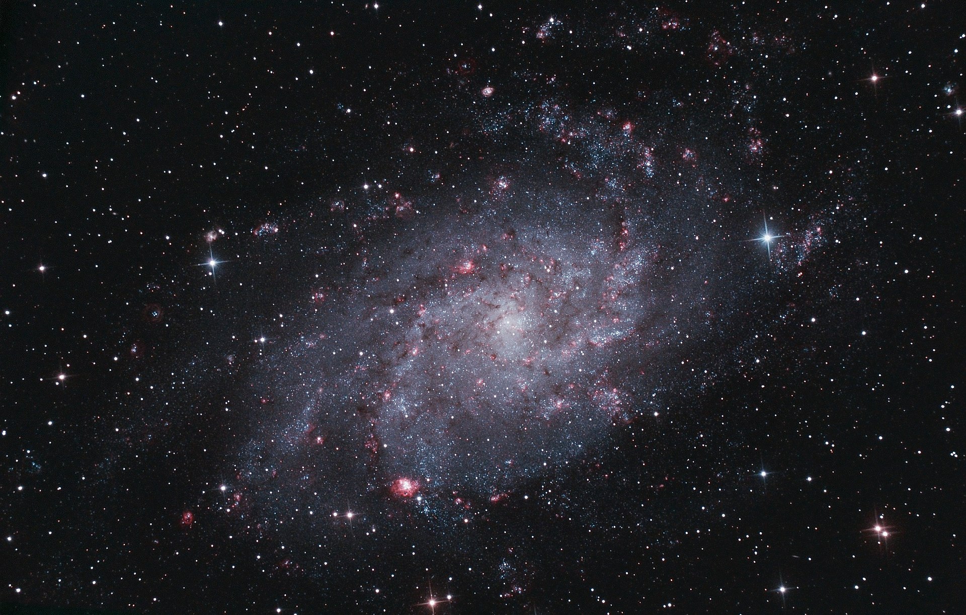
Blog #17: WS6.1, #2

2. The Hubble Classes have characteristic surface light distribution profiles. They are fairly well-described by parametrized equations in the form I(R) where I = intensity and R = distance from the center. Often each is scaled to their value at the effective radius, such that \(I_e=I(R_e)\). The most general profile is the Sérsic Profile, given by 
\(I(R)=I_eexp(-b_n[(\frac{R}{R_e})^{1/n}-1])\)
The constant \(b_n\) depends on the shape parameter n. n = 4 gives rise to the famous \(r^{1/4}\)-law, or the de Vaucoleur Profile, which approximates elliptical and the bulge of spiral galaxies. n = 1, on the other hand, is equivalent to a simple exponential profile, which often corresponds with the outskirts of spiral galaxies. The best fit is often obtained by a combination of the functional forms. 
a) Another way to write the exponential profile is \(I(R)=I_0exp(-R/b)\), where \(I_0\) is the central surface brightness and b is a characteristic lengthscale, a constant. 
i. Describe what b is, and suggest how one might measure it for a given spiral galaxy. 

b is the scale radius of the galaxy, which is defined as the radius that contains a specific proportion of the matter in the galaxy. To measure the scale radius, you could measure the fluxes in "bins" across the galaxy, then fit those measurements to the function \(I(R)=I_0exp(-R/b)\). Since you know how far each bin is from the center of the galaxy, you should be able to calculate b.

ii. The Milky Way has an estimated b = 3.5kpc. Plot the disk surface brightness profile relative to the central brightness and indicate the location of the characteristic lengthscale from the center. 

At the scale radius, b = R, so we can solve \(I(R)=I_0exp(-b/b)\). 

\(I(b)=I_0e^{-1}\)

\(I(b)=\frac{I_0}{e}\) 

iii. Assuming the entire Milky Way (including the central bulge) can be described by this profile, and that it is circularly symmetric. Approximately what fraction of all its stars are interior to the Sun (at 8kpc)? 

To find the fraction of the stars that are interior to the sun, we want to divide the total intensity in the sphere with radius = 8kpc by the total intensity of the Milky Way, regardless of radius. To find these total intensities, we can integrate the intensity function over the desired range. 

The intensity interior to the Sun: 

\(\int_{0}^{8}I(r)dr=I_0\int_{0}^{8}e^{-r/b}dr=-I_0be^{-r/b}|^8_0\)

The intensity of the entire Milky Way: 

\(\int_{0}^{\infty}I(r)dr=I_0\int_{0}^{\infty}e^{-r/b}dr=-I_0be^{-r/b}|^{\infty}_0\)

We can then take a ratio (thus canceling out the constants): 

\(\frac{e^{-r/b}|^8_0}{e^{-r/b}|^{\infty}_0}\)

Finally, we can evaluate: 

\(\frac{e^{-8/b}-e^0}{e^{-\infty/b}-e^0}=\frac{e^{-8/b}-1}{-1}=1-e^{-8/b}\) of the stars in the Milky Way are interior to the Sun. 

Blog #16: The Great Debate

The Great Debate Between Shapley and Curtis

In 1920, Heber Curtis and Harlow Shapley, two notable astronomers at the time, debated the size and the constitution of the universe. Curtis argued that the universe contained many galaxies, whereas Shapley believed that the universe only contained one galaxy. They each based parts of their arguments on what were then called "spiral nebulae."

Consistent with his views of the universe's size, Curtis thought the spiral nebulae were located outside of our own Galaxy. He thought the Galaxy was small (compared to Shapley's estimate) and that the nebulae, which he believed to be about the same size as the Galaxy, were thus located closer to us than Shapely thought. He also believed that the nebulae were similar in composition to the Milky Way, based on their appearance and their optical spectra, which were the same as that of our Galaxy.

Shapley, on the other hand, argued that they were simply large collections of dust within our Galaxy. Shapley based this idea on a rough calculation of the distance to the Magellanic Clouds, which yielded a distance smaller than the diameter of the Galaxy, and on measured rotational speeds of other nearby objects that would have to be rotating faster than the speed of light if they were outside of the Galaxy (this measured rotation speed turned out to be incorrect).

Neither of the two can really be considered as the "winner" of the debate, since each was right on some points and wrong on other points. Curtis was correct in that the nebulae are external to the Milky Way, but Shapley was right in determining that our Galaxy is larger than previously assumed and that our Sun is not at its center.

Soon after the debate, Cepheids were identified in the Andromeda Galaxy, revealing that it was a galaxy similar to our own, and far enough away to be well outside of the Milky Way. The next decade, the understanding of interstellar absorption of light allowed for better understanding of the sheer scale of the Milky Way and the position of the Sun. We now have better technology, and our understanding of galactic and extragalactic distances, as well as our knowledge of other galaxies far from our own, has improved vastly.

Sources: http://www.nasonline.org/about-nas/history/archives/milestones-in-NAS-history/the-great-debate-of-1920.html

https://en.wikipedia.org/wiki/Great_Debate_(astronomy)

http://astronomy.nmsu.edu/geas/lectures/lecture27/slide01.html

http://apod.nasa.gov/diamond_jubilee/1920/cs_why.html

http://encyclopedia2.thefreedictionary.com/Interstellar+Absorption

Blog #15: WS5.1, #3

3. A class of stars named Cepheid Variables reside in a special location in the Hertzsprung-Russell Diagram known as the instability strip. They have properties that make them crucial to the determination of large interstellar distances. 
a) Light curves (i.e. brightness time series) are often useful in studying time-variable phenomena in astrophysics. Below are a set of light curves of Cepheid Variables. Using plotting and fitting programs if necessary, find a rough relation obeyed by all the Cepheids. This relationship should relate the brightness (magnitude) of the Cepheid with another property. In other words, your relationship should have the form \(M_V = A*feature+M_0\), where A and \(M_0\) are variables you should find. 

We can use these light curves to determine the period and the \(M_V\) (mean magnitude) and of each Cepheid. 

Ashley: 

• period: 50 days
• \(M_V\): -5.7

Moiya: 

• period: 15 days
• \(M_V\): -4.4

J Arbanus: 

• period: 20 days
• \(M_V\): -4.8

Yutong: 

• period: 100 days
• \(M_V\): -6.2

Graphing \(M_V\) vs. period appears to give us a logarithmic relationship: 

So we graph \(M_V\) vs. log(period) and get a best-fit line: 

A = -2.17 and \(M_0\) = 1.925, where the "feature" is log(period): 

\(M_V = -2.17log(period)-1.925\)

b) Describe how you would measure the distance to a Cepheid.

Based on the light curve, we should know the apparent magnitude of the Cepheid. We can then plug that into the equation from question 2: 

\(d = D*10^{0.2(m-M)}\) where D = 10pc

c) Below is an image of a Cepheid Variable in the Large Magellanic Cloud. Determine its period, mean absolute magnitude, and distance. 

The period is the distance between the two peaks, which is approximately 5 weeks or 35 days. 

We can calculate the mean absolute magnitude using the equation from part a.

\(M_V = -2.17log(35)-1.925 = -5.28\) 

Using this absolute magnitude, we can calculate the distance using the equation from part b, where m is the mean apparent magnitude of 15.6 and M is the mean absolute magnitude of -5.28. 

\(d = 10*10^{0.2(15.6+5.28)} = 1.5 * 10^5pc \rightarrow 150kpc\)

Blog #14: WS5.1, #2

2. a) Suppose you are observing two stars, Star A and Star B. Star A is 3 magnitudes fainter than Star B. How much longer do you need to observe Star A to collect the same amount of energy in your detector as you do for Star B? 

If the fluxes of Star A and Star B are \(F_A\) and \(F_B\), their magnitudes (\(m_A\) and (\m_B\)) should obey the relationship \(\frac{F_A}{F_B} = 2.5^{m_B-m_A}\). Since Star B is 3 magnitudes brighter, \(\frac{F_A}{F_B} = 2.5^3 = 15.6\). We'd need to observe Star A for about 16 times longer to get the same amount of energy.

b) Stars have both an apparent magnitude, m, which is how bright they appear from the Earth. They also have an absolute magnitude, M, which is the apparent magnitude a star would have at D = 10pc. How does the apparent magnitude, m, of a star with absolute magnitude M, depend on its distance, d, from you? 

The flux of the star at distance d would be \(F_d = \frac{L}{4\pi d^2}\), so the flux at the standard distance of 10 pc would be \(F_D = \frac{L}{4\pi (10pc)^2}\). We can then take the ratio of the two and use that to solve for m.
\(10^{0.4(m-M)} = \frac{F_D}{F_d}\) which simplifies to \(\frac{d^2}{D^2}\)
\(0.4(m-M) = log(\frac{d^2}{D^2})\)
\(m-M = 2.5log(\frac{d^2}{D^2})\)
\(m = M+5log(\frac{d}{D})\) where D = 10pc.

c) What is the star's parallax in terms of its apparent and absolute magnitude? 

We can rewrite the equation above to solve for d instead of m.
\(d = D*10^{0.2(m-M)}\)
We can then plug this into the parallax equation, \(\theta = \frac{1AU}{d}\).
\(\theta = \frac{1AU}{D*10^{0.2(m-M)}}\) where D = 10pc.